4. Neural Networks

Taught by: Dat Doan, Alex Ganose

The start of this notebook was inspired by the ML for Materials course developed by Prof. Aron Walsh.

Getting started

Welcome to the third practical session! As always, the notebook is designed to be run online directly in your browser by clicking the rocket icon on the top right and selecting Live Code.

Outline

This workshop will cover the following content:

1. The perceptron

2. Multi-layer perceptrons

3. NNs with PyTorch

4. Image classification

5. Convolutional neural networks

Artificial Neural Networks

Artificial neural networks are a class of machine learning models that are inspired by the structure and function of the human brain.

A short history of neural networks:

• 1943: McCulloch and Pitts propose a mathematical model of a neuron in the landmark paper “A logical calculus of the ideas immanent in nervous activity”.

• 1958: Rosenblatt introduces the perceptron, a simple neural network model.

• Dark years: Neural networks fall out of favor due to limitations in training algorithms and computational power. Funding for neural network research is cut.

• 1980s: Neural networks experience a resurgence due to the development of backpropagation and the increasing availability of computational resources.

• 1980: Hopfield introduces the Hopfield network, a type of recurrent neural network.

• 1986: Rumelhart, Hinton, and Williams publish a paper on backpropagation, a method for training neural networks.

• 2012: AlexNet wins the ImageNet competition, demonstrating the power of deep learning.

• 2016: AlphaGo defeats the world champion Go player, demonstrating the power of deep reinforcement learning.

Neural networks have become increasingly popular in recent years due to their ability to learn complex patterns from data and make accurate predictions. They can be used to classify billions of images, translate languages in real-time, and play games at a superhuman level.

Biological vs artificial neural networks

Biological neural networks are composed of interconnected neurons that communicate with each other through electrical and chemical signals. These networks are responsible for processing information, learning, and controlling behavior.

Artificial neural networks are inspired by biological neural networks but are much simpler in structure and function. There are many different types of neural networks, each with its own architecture and set of rules for updating the weights.

Biological neurons	Artificial neurons
Composed of dendrites, a cell body and an axon.	Composed of input connections + synaptic weights, a summing junction and an activation function.
Sends signals in the form of neurotransmitters (chemicals) into the synaptic terminals	Sends signals in the form of numbers (in 1943: binary on/off) into the output connection
Activates when cell body receives a sufficient amount of signals through dendrites	Activates when sufficient number of input connections are active

The perceptron

The perceptron is the simplest form of a neural network. It is a single-layer neural network that takes in a set of inputs and produces a single output. The output is calculated by taking the dot product of the input vector and a set of weights, and passing the result through an activation function.

\[\begin{split} y = \begin{cases} 1 & \text{if } \sum_{i=1}^{n} x_i w_i + \beta > 0 \\ 0 & \text{otherwise} \end{cases} \end{split}\]

where

• \(x_i\) is the \(i\)-th input

• \(w_i\) is the \(i\)-th weight

• \(\beta\) is the bias

• \(n\) is the number of inputs

The weights are adjusted during training to minimize the error between the predicted output and the true output.

Let’s start be implementing a basic perceptron model. You should finish the perceptron function below, based on the formula for the perceptron given above.

import numpy as np

# Write a function to calculate the output of a perceptron model
def perceptron(x, w, b=0):
  """Perceptron model
  
  Args:
    x: input vector (array with 2 elements)
    w: weights vector (array with 2 elements)
    b: bias term
  """

Answer

The easiest solution is to use the numpy `dot` function to take the dot product between the weights and inputs. The finished code could look something like this:

def perceptron(x, w, b=0):
  """Perceptron model
  
  Args:
    x: input vector (array with 2 elements)
    w: weights vector (array with 2 elements)
    b: bias term
  """
  h = np.dot(x, w) + b
  return 1 if h > 0 else 0

We can play around with the behaviour of the perceptron by running it on different inputs.

print("The output for x = (1,  1)  w = (1,  1) is", perceptron([1, 1], [1, 1]))
print("The output for x = (0,  0)  w = (0,  0) is", perceptron([0, 0], [0, 0]))
print("The output for x = (-1, 0)  w = (1,  0) is", perceptron([-1, 0], [1, 0]))
print("The output for x = (-1, 0)  w = (-1, 0) is", perceptron([-1, 0], [-1, 0]))

We have written a simple code to visualise the performance of the perceptron on the domain of -1 to 1. There are two dummy features (scaled temperature and scaled pressure) and we assign the model outputs to “Gas phase” (1) or “Liquid phase” (0).

import matplotlib.pyplot as plt
from matplotlib.patches import Patch

weights = (-0.25, 0.9)
bias = 0

# Create data points for visualisation
n_points = 200
temp = np.linspace(-1, 1, n_points)
pressure = np.linspace(-1, 1, n_points)
X1, X2 = np.meshgrid(temp, pressure)

# run the perceptron on the data points
predicted_labels = [
    perceptron(x, weights, bias)
    for x in zip(X2.flat, X1.flat)
]
predicted_labels = np.array(predicted_labels).reshape(n_points, n_points)

fig, ax = plt.subplots()
ax.contourf(X1, X2, predicted_labels, alpha=0.2, levels=[-1, 0, 1], colors=('blue', 'orange'))
ax.set(xlabel='Scaled Temperature', ylabel='Scaled Pressure', title='Perceptron Model Phase Diagram')
ax.legend(handles=[Patch(color='blue', label='Liquid'), Patch(color='orange', label='Gas')])
ax.grid()
plt.show()

You can play around with the weights and bias as the top of the cell to see how it changes the behaviour.

Multi-Layer Perceptrons

A multi-layer perceptron (MLP) is a neural network with one or more layers of perceptrons. The output of one layer of perceptrons is used as input for the next layer. The first layer is called the input layer, the last layer is called the output layer, and the layers in between are called hidden layers. When the number of layers becomes large (most commonly tens, or even hundreds nowadays), the model is usually considered a deep neural network, one of the most powerful class of machine learning algorithms today and is known commonly as Deep Learning.

We can expand our previous model by building a small multi-layer perceptron with one hidden layer. To make the model more flexible, we will use the sigmoid activation function instead of the step function. The sigmoid function is defined as:

\[ \sigma(x) = \frac{1}{1 + e^{-x}} \]

We can define this in python as:

def sigmoid(x):
  return 1 / (1 + np.exp(-x))

print("The output for (-1) is", sigmoid(-1))
print("The output for (0) is", sigmoid(0))
print("The output for (1) is", sigmoid(1))
print("The output for (10000) is", sigmoid(10000))

Let’s now create a simple neural network using the sigmoid activation function.

• The first layer of the model is the input layer (in our case containing two features).

• The second layer is the hidden layer with two perceptrons using the sigmoid activation function.

• The third layer is the output layer with one perceptron using the sigmoid activation function.

This can be represented graphically as:

We have labelled the neurons 1, 2, and 3. Mathemetically, the model can be defined as:

\[\begin{split} \begin{align*} \mathbf{h} & = \begin{bmatrix} \sigma(\mathbf{x} \cdot \mathbf{w}_1 + \beta_1) \\ \sigma(\mathbf{x} \cdot \mathbf{w}_2 + \beta_2) \end{bmatrix} \\ y &= \sigma(\mathbf{h} \cdot \mathbf{w}_3 + \beta_3) \end{align*} \end{split}\]

where:

• \(\mathbf{x}\) are the input features

• \(\mathbf{w}_i\) are the weights for the \(i\)-th neuron

• \(\beta_i\) is the bias for the \(i\)-th neuron

• \(\mathbf{h}\) is the output of the hidden layer

• \(y\) is the output of the model.

You should finish the neural_network function below, based on the formulae given above.

def neural_network(x, w1, w2, w3, b1=0, b2=0, b3=0):
  """Neural network model
  
  Args:
    x: input vector (array with 2 elements)
    w1, w2, w3: weights vectors (arrays with 2 elements)
    b1, b2, b3: bias terms
  """

Answer

Again, the easiest solution is to use the numpy `dot` function to take the dot product between the weights and inputs. The finished code could look something like this:

def neural_network(x, w1, w2, w3, b1=0, b2=0, b3=0):
  """Neural network model
  
  Args:
    x: input vector (array with 2 elements)
    w1, w2, w3: weights vectors (arrays with 2 elements)
    b1, b2, b3: bias terms
  """
  h = [
      sigmoid(np.dot(x, w1) + b1),
      sigmoid(np.dot(x, w2) + b2)
  ]
  return sigmoid(np.dot(h, w3) + b3)

If you’re unsure about the code, please speak to one of the course assistants.

Once you’re happy with your code, you can see what it predicts using the cell below.

weights1 = [ 3.8430335, -3.17603404] 
weights2 = [-0.5338159, -2.88928327]
weights3 = [-2.66952744,  3.82808745]
bias1 = 0
bias2 = 0
bias3 = 0

# run the network on the data points
predicted_labels = [
    neural_network(x, weights1, weights2, weights3, bias1, bias2, bias3)
    for x in zip(X2.flat, X1.flat)
]
predicted_labels = np.array(predicted_labels).reshape(n_points, n_points)

def plot_results(predicted_labels):
    fig, ax = plt.subplots()
    cont = ax.contourf(X1, X2, predicted_labels, alpha=0.5, levels=np.linspace(0, 1, 11), cmap='coolwarm')
    ax.set(xlabel='Scaled Temperature', ylabel='Scaled Pressure', title='Two-Layer NN: Phase Diagram')
    plt.colorbar(cont, label='Phase Probability')
    ax.grid()
    plt.show()

plot_results(predicted_labels)

With just two layers and the sigmoid activation function, we’re able to describe a wide range of relatively complex functions. You can play around with the weights and biases to get a feel for how the function behaves.

NNs with PyTorch

In practice, you won’t be coding your neural networks from scratch. Instead, you’ll use libraries like PyTorch, TensorFlow, or JAX, which provide efficient implementations of neural network layers, optimizers, and other tools. In this course, we’ll be using Pytorch, which is open-source machine learning library primarily developed by Facebook’s AI Research lab (FAIR).

Let’s build the same model as before using PyTorch. We’ll use the Sequential class which builds a simple net where each layer is applied in sequence, with the output of each layer passed as input to the next layer. We’ll make use of the Linear layer, where we must define the number of input features and output features. For example, nn.Linear(2, 2) creates a linear layer with 2 input features and 2 output features. The Sigmoid activation function is applied after each linear layer.

import torch.nn as nn

model = nn.Sequential(
    nn.Linear(2, 2),
    nn.Sigmoid(),
    nn.Linear(2, 1),
    nn.Sigmoid()
)
model

Take a second to make sure you understand this code, and that you’re happy with the numbers of inputs/outputs in each layer.

As an example, we now use our model in place of the neural_network function we defined before. Note, we have to set the weights of the model to match what we used before. Normally we’d either load these from a file or find them through model training.

import torch

# set the model weights to the values we used before
model.load_state_dict({
    '0.weight': torch.tensor([[ 3.8430335, -3.17603404],
                              [-0.5338159, -2.88928327]]),
    '0.bias': torch.tensor([0, 0]),
    '2.weight': torch.tensor([[-2.66952744,  3.82808745]]),
    '2.bias': torch.tensor([0])
})

predicted_labels = [
    model(torch.tensor(x, dtype=torch.float32))
    for x in zip(X2.flat, X1.flat)
]
predicted_labels = torch.tensor(predicted_labels).reshape(n_points, n_points)

plot_results(predicted_labels)

The result is exactly the same as before, but now we are using a PyTorch model.

Image classification

So far we only been working with simple toy models. In this section, we will see how to build a more complex model to classify images. We will use the Fashion-MNIST dataset, which is a collection of 28x28 grayscale images of 10 different classes of clothing items. The dataset is available in the torchvision package, which provides a collection of datasets and models for computer vision tasks.

The classes of the dataset correspond to:

Index	Category
0	T-shirt/top
1	Trouser
2	Pullover
3	Dress
4	Coat
5	Sandal
6	Shirt
7	Sneaker
8	Bag
9	Ankle boot

First let’s download the dataset. It has already been split into the training and testing sets but we need to download them separately. Furthermore, the data is stored as pixels with values from 0 to 255. However, we need to normalise the data first so that the numbers vary from -1, 1. In general, normalisation is essential to ensure your model trains successfully.

from torchvision.datasets import FashionMNIST
import torchvision.transforms as transforms

transform = transforms.Compose([
    transforms.ToTensor(),                # Convert image to PyTorch tensor
    transforms.Normalize((0.5,), (0.5,))  # Normalize the image
])

train_data = FashionMNIST(root='./data', train=True, download=True, transform=transform)
test_data = FashionMNIST(root='./data', train=False, download=True, transform=transform)

# only load the first 500 (train) and 100 (test) images of each dataset
train_data.data = train_data.data[:500]
train_data.targets = train_data.targets[:500]

# split the train data into a training and validation set
train_data, val_data = torch.utils.data.random_split(train_data, [400, 100])

test_data.data = test_data.data[:100]
test_data.targets = test_data.targets[:100]

classes = test_data.classes

Confirm the dataset sizes:

print("Training set size:", len(train_data))
print("Validation set size:", len(val_data))
print("Test set size:", len(test_data))

Put the data into a DataLoader. This is a PyTorch class that helps with batching and shuffling data.

from torch.utils.data import DataLoader

train_dataloader = DataLoader(train_data, batch_size=4, shuffle=True)
val_dataloader = DataLoader(val_data, batch_size=4, shuffle=False)
test_dataloader = DataLoader(test_data, batch_size=4, shuffle=False)

Lets plot a few images from the dataset:

from torchvision.utils import make_grid

def imshow(img):
    img = img / 2 + 0.5  # unnormalize
    plt.imshow(img.permute(1, 2, 0))
    plt.show()

# get a batch of 4 images
images, labels = next(iter(train_dataloader))

imshow(make_grid(images))
print(' '.join(classes[l] for l in labels))

Now we can build our model. We’ll again use the Sequential model from Pytorch. We’ll make an MLP with 2 hidden layers with the ReLU activation function. The final layer will use a softmax function to get class probabilities.

model = nn.Sequential(
    nn.Flatten(),           # (N, 1, 28, 28) -> (N, 784)
    nn.Linear(28*28, 256),  # (N, 784) -> (N, 256)
    nn.ReLU(), 
    nn.Linear(256, 128),    # (N, 256) -> (N, 128)
    nn.ReLU(),
    nn.Linear(128, 10),     # (N, 128) -> (N, 10)
    nn.LogSoftmax(dim=1)
)

model

We can check the number of trainable parameters:

def count_parameters(model):
    return sum(p.numel() for p in model.parameters() if p.requires_grad)

print(f'The model has {count_parameters(model):,} trainable parameters')

Next, we need to specify the loss function and optimiser:

• Loss function — This measures how accurate the model is during training. You want to minimize this function to “steer” the model in the right direction. Here we use cross entropy loss.

• Optimiser — This is how the model weights are updated based on the data it sees and its loss function. Here we use stochastic gradient descent. We have to pass the model parameters into the optimiser so it can update them.

import torch.optim as optim

criterion = nn.CrossEntropyLoss()
optimizer = optim.SGD(model.parameters(), lr=0.001, momentum=0.9)

Finally, we can train the model. Training a neural network involves iteratively updating its weights to minimize the loss function. This process is typically achieved using gradient descent optimization algorithms. Here’s an in-depth explanation of the training loop:

1. Epochs: An epoch represents one complete forward and backward pass of all the training examples. The number of epochs (num_epochs) is the number of times the learning algorithm will work through the entire training dataset. Usually a custom hyperparameter.

2. Model Training Mode: Neural networks can operate in different modes - training and evaluation. Some layers, like dropout, behave differently in these modes. Setting the model to training mode ensures that layers like dropout function correctly.

3. Batch Processing: Instead of updating weights after every training example (stochastic gradient descent) or after the entire dataset (batch gradient descent), we often update weights after a set of training examples known as a batch.

4. Zeroing Gradients: In PyTorch, gradients accumulate by default. Before calculating the new gradients in the current batch, we need to set the previous gradients to zero.

5. Forward Pass: The input data (images) are passed through the network, layer by layer, until we get the output. This process is called the forward pass.

6. Calculate Loss: Once we have the network’s predictions (outputs), we compare them to the true labels using a loss function. This gives a measure of how well the network’s predictions match the actual labels.

7. Backward Pass: To update the weights, we need to know the gradient of the loss function with respect to each weight. The backward pass computes these gradients.

8. Update Weights: The optimizer updates the weights based on the gradients computed in the backward pass.

This loop (forward pass, loss computation, backward pass, weight update) is repeated for every batch in the dataset, and the whole process is repeated for the specified number of epochs.

At the same time, we also evaluate the performance of the model on the validation set at the end of each epoch.

# Number of complete passes through the dataset
num_epochs = 10

# keep track of the loss for each epoch
train_losses = []
val_losses = []

# Start the training loop
for epoch in range(num_epochs):
    # Set the model to training mode
    model.train()

    # Initialize a variable to keep track of the cumulative loss for this epoch
    train_loss = 0.0
    
    # Iterate over each batch of the training data
    for images, labels in train_dataloader:
        # Clear the gradients from the previous iteration
        optimizer.zero_grad()
        
        # Forward pass: Pass the images through the model to get the predicted outputs
        outputs = model(images)
        
        # Compute the loss between the predicted outputs and the true labels
        loss = criterion(outputs, labels)
        
        # Backward pass: Compute the gradient of the loss w.r.t. model parameters
        loss.backward()
        
        # Update the model parameters
        optimizer.step()

        # Add the loss for this batch to the epoch loss
        train_loss += loss.item()
    
    # Iterate over the validation data and compute the loss
    model.eval()
    val_loss = 0.0

    # turn off gradients since we are in the evaluation mode
    with torch.no_grad():
        for images, labels in val_dataloader:
            # Forward pass: Pass the images through the model to get the predicted outputs
            outputs = model(images)

            # Compute the loss between the predicted outputs and the true labels
            loss = criterion(outputs, labels)

            # Add the loss for this batch to the validation loss
            val_loss += loss.item()

    train_losses.append(train_loss/len(train_dataloader))
    val_losses.append(val_loss/len(val_dataloader))
    print(f"Epoch [{epoch+1}/{num_epochs}], Train loss: {train_losses[-1]:.4f}, Val loss: {val_losses[-1]:.4f}")

We can plot the performance of the model as a function of epochs:

fig, ax = plt.subplots()
ax.plot(train_losses, label="train")
ax.plot(val_losses, label="val")
ax.set(xlabel='Epoch', ylabel='Loss')
ax.legend()
plt.show()

It looks like our train loss dropped rapidly at first and was still decreasing slowly. The validation loss also dropped at first but seems to have flattened out. This gives an indication that the model is beginning to overfit to the data.

To check the performance of our model, we should look at the performance on the test set. Here, we don’t want to compute the model gradients as we are no longer training, so we’ll use torch.no_grad().

# Test the model
model.eval()

correct = 0
with torch.no_grad():
    for images, labels in test_dataloader:
        # Get the class probabilities
        output = model(images)

        # Get the class with the maximum probability as the predicted class
        _, predicted = torch.max(output, 1)
        
        # Count the number of correct predictions
        correct += (predicted == labels).sum().item()

accuracy = correct / len(test_data)
print(f"Accuracy on the test set: {accuracy * 100:.2f}%")

Let’s see what this looks like against the actual data:

images, labels = next(iter(test_dataloader))
output = model(images)
_, predicted = torch.max(output, 1)

imshow(make_grid(images))
print('GroundTruth: ', ' '.join(classes[l] for l in labels))
print('Predicted: ', ' '.join(classes[p] for p in predicted))

Convolutional Neural Networks

In the previous sequential model, the first layer is the flatten layer with shape 784 x 1 (28 x 28). This means that we lose information about how the image is structured. Convolutional neural networks (CNNs) are able to successfully capture the spatial and temporal dependencies in an image through the application of relevant filters.

Neurons in the first convolutional layer are not connected to every single pixel in the input image, but only to pixels in their receptive fields. In turn, each neuron in the second convolutional layer is connected only to neurons located within a small square in the first layer. This architecture allows the network to concentrate on small low-level features in the first hidden layer, then assemble them into larger higher-level features in the next hidden layer, and so on.

Key building blocks of CNNs

A typical CNN architecture consists of:

• Convolutional Layers: Apply convolution operation on the input layer to detect features.

• Activation Layers: Introduce non-linearity to the model (typically ReLU).

• Pooling Layers: Perform down-sampling operations to reduce dimensionality.

• Fully Connected Layers: After several convolutional and pooling layers, the high-level reasoning in the neural network happens via fully connected layers.

Here’s an example:

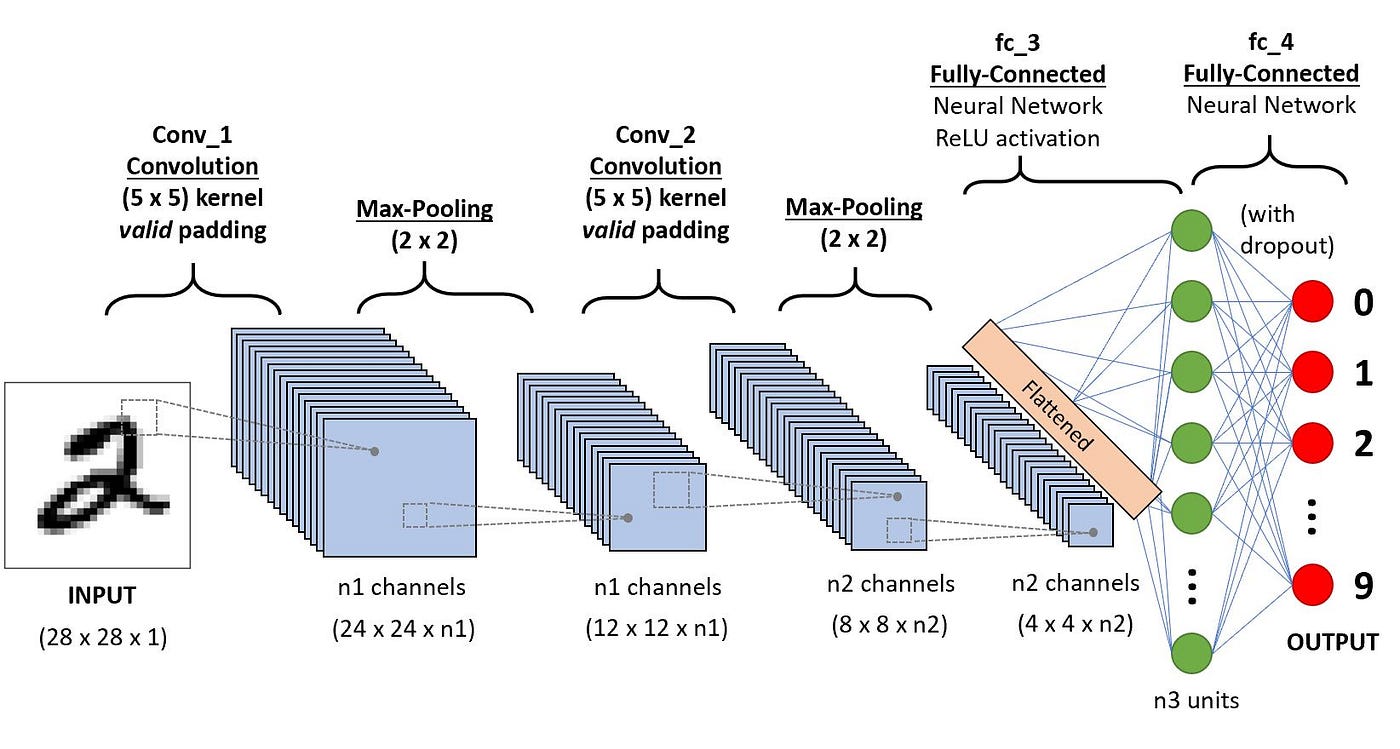
The key parameters to be aware of for the different layers are:

Conv2d

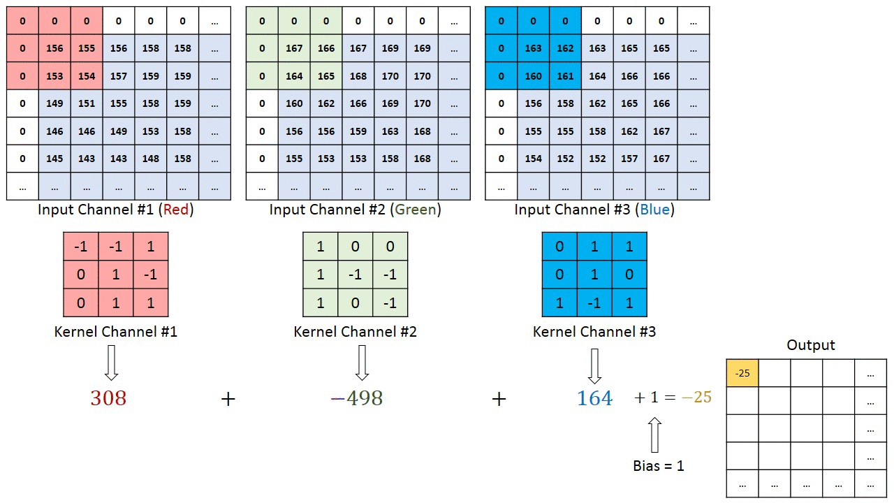
This layer applies a 2D convolution to the input tensor. For example, nn.Conv2d(1, 32, 3):

• The first argument is the number of input channels.

• The second argument is the number of output channels. This represents the number of filters that are applied to the input tensor. Each filter can learn to detect different features in the input tensor.

• The third argument is the kernel size (the size of the filter). E.g., above we use a kernel size of 3, which results in a 3x3 filter. The output tensor will have the specified number of output channels and the *size of the input tensor will be reduced by 2 in each dimension.

MaxPool2d

This layer applies 2D max pooling to the input tensor. For example, `nn.MaxPool2d(2)

• The argument is the size of the filter that is applied to the input tensor. In this case, we are using a filter size of 2, which means that the filter will be a 2x2 filter. The output tensor will have the same number of channels as the input tensor and the size of the input tensor will be reduced by half in each dimension.

Let’s design a basic CNN for our dataset.

model = nn.Sequential(
    nn.Conv2d(1, 32, 3),     # (N, 1, 28, 28) -> (N, 32, 26, 26)
    nn.ReLU(),
    nn.MaxPool2d(2),         # (N, 32, 26, 26) -> (N, 32, 13, 13)
    nn.Conv2d(32, 64, 3),    # (N, 32, 13, 13) -> (N, 64, 11, 11)
    nn.ReLU(),
    nn.MaxPool2d(2),         # (N, 64, 11, 11) -> (N, 64, 5, 5)
    nn.Flatten(),            # (N, 64, 5, 5) -> (N, 1600)
    nn.Linear(64*5*5, 128),  # (N, 1600) -> (N, 128)
    nn.ReLU(),               
    nn.Linear(128, 10),      # (N, 128) -> (N, 10)
    nn.LogSoftmax(dim=1)
)
print(model)
print(f'The model has {count_parameters(model):,} trainable parameters')

Now let’s train the model, exactly the same as we did before:

# define the loss function and the optimizer
criterion = nn.CrossEntropyLoss()
optimizer = optim.SGD(model.parameters(), lr=0.001, momentum=0.9)

num_epochs = 10
train_losses = []
val_losses = []

for epoch in range(num_epochs):

    # train the model
    model.train()
    train_loss = 0.0
    for images, labels in train_dataloader:
        optimizer.zero_grad()
        outputs = model(images)
        loss = criterion(outputs, labels)
        loss.backward()
        optimizer.step()
        train_loss += loss.item()
    
    # evaluate the model
    model.eval()
    val_loss = 0.0
    with torch.no_grad():
        for images, labels in val_dataloader:
            outputs = model(images)
            loss = criterion(outputs, labels)
            val_loss += loss.item()
    
    train_losses.append(train_loss/len(train_dataloader))
    val_losses.append(val_loss/len(val_dataloader))
    print(f"Epoch [{epoch+1}/{num_epochs}], Train loss: {train_losses[-1]:.4f}, Val loss: {val_losses[-1]:.4f}")

Plot the training metrics:

fig, ax = plt.subplots()
ax.plot(train_losses, label="train")
ax.plot(val_losses, label="val")
ax.set(xlabel='Epoch', ylabel='Loss')
ax.legend()
plt.show()

And now evaluate the accuracy:

# Test the model
model.eval()

correct = 0
with torch.no_grad():
    for images, labels in test_dataloader:
        # Get the class probabilities
        output = model(images)

        # Get the class with the maximum probability as the predicted class
        _, predicted = torch.max(output, 1)
        
        # Count the number of correct predictions
        correct += (predicted == labels).sum().item()

accuracy = correct / len(test_data)
print(f"Accuracy on the test set: {accuracy * 100:.2f}%")

In class challenge

Since CNNs work better for more complex images, let’s now build an image classifier with coloured pictures.

We’ll use the CIFAR-10 dataset, which consists of 32x32 colour images in 10 classes, with 6,000 images per class. Becaue the images are in colour (RGB), each image has 3 channels. The classes for the dataset are:

Label	Description
0	airplane
1	automobile
2	bird
3	cat
4	deer
5	dog
6	frog
7	horse
8	ship
9	truck

We’ll first load the dataset and only use the first 5000 images for training and the first 1000 images for testing.

from torchvision.datasets import CIFAR10

transform = transforms.Compose([
    transforms.ToTensor(),
    transforms.Normalize((0.5, 0.5, 0.5), (0.5, 0.5, 0.5))
])

train_data = CIFAR10(root='./data', train=True, download=True, transform=transform)
test_data = CIFAR10(root='./data', train=False, download=True, transform=transform)

# only load the first 5000 (train) and 1000 (test) images of each dataset
train_data.data = train_data.data[:500]
train_data.targets = train_data.targets[:500]

# split the train data into a training and validation set
train_data, val_data = torch.utils.data.random_split(train_data, [400, 100])

test_data.data = test_data.data[:100]
test_data.targets = test_data.targets[:100]

classes = test_data.classes

# create data loaders
train_dataloader = DataLoader(train_data, batch_size=4, shuffle=True)
val_dataloader = DataLoader(val_data, batch_size=4, shuffle=False)
test_dataloader = DataLoader(test_data, batch_size=4, shuffle=False)

print("Training set size:", len(train_data))
print("Validation set size:", len(val_data))
print("Test set size:", len(test_data))

Plot the first 4 images of the training set and their labels.

images, labels = next(iter(train_dataloader))
imshow(make_grid(images))
print(" ".join(classes[l] for l in labels))

# 3, 2, 1, code!
# remeber to change the input shape and number of channels in your first and linear layers

Answer

The following model can be used. The only changes from the previous model is that the number of input channels for the first convolution has been changed from 1 to 3, and the input size of the linear layer has been changed to 2304. The second change is required since the images have different initial dimensions. Following the pooling and convolution operations through gives you this final answer.

model = nn.Sequential(
    nn.Conv2d(3, 32, 3),     # (N, 3, 32, 32) -> (N, 32, 30, 30)
    nn.ReLU(),
    nn.MaxPool2d(2),         # (N, 32, 30, 30) -> (N, 32, 15, 15)
    nn.Conv2d(32, 64, 3),    # (N, 32, 13, 13) -> (N, 64, 13, 13)
    nn.ReLU(),
    nn.MaxPool2d(2),         # (N, 64, 13, 13) -> (N, 64, 6, 6)
    nn.Flatten(),            # (N, 64, 6, 6) -> (N, 2304)
    nn.Linear(64*6*6, 128),  # (N, 2304) -> (N, 128)
    nn.ReLU(),               
    nn.Linear(128, 10),      # (N, 128) -> (N, 10)
    nn.LogSoftmax(dim=1)
)

The rest of the training and evaluation code can be used as before.

Features of molecules and materials

For chemical problems, we often need to work with molecular or crystal structures. These structures can be represented in many ways, such as SMILES strings, molecular graphs, or 3D coordinates. However, these representations are not directly usable by neural networks. Instead, we need to extract features that can be used as input to a neural network. This process is called featurization.

Molecules

Simplified molecular-input line-entry system (SMILES) are a way of representing molecules as text. For example:

CH3−N=C=O CN=C=O

Cu²⁺SO₂⁻ [Cu+2].[O-]S(=O)(=O)[O-]

CN1CCC[C@H]1c2cccnc2

OCCc1c(C)[n+](cs1)Cc2cnc(C)nc2N

We can generate molecular fingerprints (features) from these SMILES strings using the RDKit library. For example, using Morgan fingerprints, a populator method to turn molecules of any shape into fixed-length vectors.

Let’s use caffeine as an example (CN1C=NC2=C1C(=O)N(C(=O)N2C)C). First, we create a molecule object from the SMILES string:

from rdkit.Chem import MolFromSmiles

mol = MolFromSmiles('CN1C=NC2=C1C(=O)N(C(=O)N2C)C')
mol

Next, we can generate the morgan fingerprint and the RDKit fingerprint:

from rdkit.Chem import rdFingerprintGenerator

# Morgan Fingerprint
morgan_gen = rdFingerprintGenerator.GetMorganGenerator(radius=4)
morgan_fp = morgan_gen.GetFingerprint(mol)
morgan_fp_np = np.array(morgan_fp)
print("Morgan Fingerprint:", morgan_fp_np, "Shape:", morgan_fp_np.shape)

# RDK Fingerprint
rdkit_gen = rdFingerprintGenerator.GetRDKitFPGenerator()
rdkit_fp = rdkit_gen.GetFingerprint(mol)
rdkit_fp_np = np.array(rdkit_fp)
print("RDK Fingerprint:", rdkit_fp_np, "Shape:", rdkit_fp_np.shape)

Crystals

Features for crystal structures and compositions can be generated using the matminer library. Here is an example of how to generate elemental features for a composition, specifically the Magpie elemental features.

First, we create a Composition object using the pymatgen library:

from pymatgen.core import Composition

comp = Composition("Fe2O3")
comp

Next, we can generate the features using matminer.

from matminer.featurizers.composition import ElementProperty

magpie_gen = ElementProperty.from_preset(preset_name="magpie")
magpie_fp = np.array(magpie_gen.featurize(comp))

print("Magpie Features:", magpie_fp.round(2).tolist(), "Shape:", magpie_fp.shape)
print("Magpie Feature Names:", magpie_gen.feature_labels()) 

We can also generate structures for crystal structures, starting from a pymatgen Structure object:

from pymatgen.core import Structure

structure = Structure.from_spacegroup(
    sg='Fm-3m',
    species=['Na+', 'Cl-'],
    lattice=[[5.64, 0, 0], [0, 5.64, 0], [0, 0, 5.64]],
    coords=[[0, 0, 0], [0.5, 0.5, 0.5]]
)
structure

Next, we generate the site stats fingerprint which summarises the different coordination environments in the structure:

from matminer.featurizers.structure import SiteStatsFingerprint

ssf_gen = SiteStatsFingerprint.from_preset("CrystalNNFingerprint_ops")
ssf_fp = np.array(ssf_gen.featurize(structure))

print("Structure Features:", ssf_fp, "Shape:", ssf_fp.shape)
print("Structure Feature Names:", ssf_gen.feature_labels()) 

Many more options are available. See the matminer documentation for more details.

Additional reading

• This notebook can be complimented with Chapters 3 and 4 of Understanding Deep Learning for more comprehensive to introduction to neural networks.

• The videos on neural networks by 3Brown1Blue can also help develop a more intuitive understanding.